Ok, here we go…
I made small scripts that basically just expose the different inbuilt functions and add some basic scale and rotation controls:
Voronoi cells
# Basic usage of the inbuilt seexpr voronoi function.
# This just exposes each of the variables in the voronoi function for editing. Also adds rotation and scaling.

# UV vector manipulation
# ----------------------

# Construction of the UV vector. $u and $v are the normalized x and y coordinates for the image. This gives non-square results by default, so we calculate the ratio and then multiply the relevant dimension with said ratio to get a square result from the algorithms.
# The zCoordinate can be set manually in many of the inbuilt noise functions, as these produce 3d noise, but we have a 2d plane. So allowing people to manipulate the last dimension manually allows them to access other slices of the 3d noise.

$ratio = $h/$w;
$zCoord = 0; #0.0, 1.0
$uv = [$u, $v*$ratio, zCoord];

# We multiply the subdivisions with the uv vector to give a sense of zooming out.

$subdivisions = 10; # 1, 100;
$uv *= $subdivisions;

# We also rotate the uv coordinate around the z-axis, [0,0,1].

$rotation = 0; #0, 359;
$uv = rotate($uv, [0,0,1], rad(rotation));


# Voronoi Function
# ----------------

# The type of voronoi algorithm as explain in the manual.
$type = 2; #1, 5

# The jitter, low jitter gives almost grid like appearance, high jitter a
$jitter = 1; #0.0, 1.0

# Some variables for introducing some fractal brownian motion into the voronoi cells.

# The strength of the FBM effect.
$fbmScale = 0;

# Controls the frequencies.
$fbmOctaves = 4; #0, 10

# Spacing between the frequencies - a value of 2 means each octave is twice the previous frequency.
$fbmLacunarity = 2; #0, 10;

# controls how much each frequency is scaled relative to the previous frequency.
$fbmGain = 0.5; #0, 10.0

# Finally we input all the variables into the function to get a factor.
$fac = voronoi($uv, $type, $jitter, $fbmScale, $fbmOctaves, $fbmLacunarity, $fbmGain);


# Color
# -----
# We put the factor into a gradient to get the color.

$color = ccurve($fac,0,[0.141,0.059,0.051],4,0.709957,[1,1,0],4,1,[0.976,0.976,0.976],4,0.212121,[0.333333,0,0],4,0.519481,[1,0.333333,0],4);

# return the color.
$color
Perlin Noise 1983
# Basic usage of the inbuilt seexpr noise function.
# This is based on the original 1983 perlin noise.

# UV vector manipulation
# ----------------------

# Construction of the UV vector. $u and $v are the normalized x and y coordinates for the image. This gives non-square results by default, so we calculate the ratio and then multiply the relevant dimension with said ratio to get a square result from the algorithms.
# The zCoordinate can be set manually in many of the inbuilt noise functions, as these produce 3d noise, but we have a 2d plane. So allowing people to manipulate the last dimension manually allows them to access other slices of the 3d noise.

$ratio = $h/$w;
$zCoord = 0; #0.0, 1.0
$uv = [$u, $v*$ratio, zCoord];

# We multiply the subdivisions with the uv vector to give a sense of zooming out.

$subdivisions = 67; # 1, 100;
$uv *= $subdivisions;

# We also rotate the uv coordinate around the z-axis, [0,0,1].

$rotation = 0; #0, 359;
$uv = rotate($uv, [0,0,1], rad(rotation));


# Noise Function
# ----------------


# Finally we input all the UV into the function to get a factor.
$fac = noise($uv);


# Color
# -----
# We put the factor into a gradient to get the color.

$color = ccurve($fac,0,[0.141,0.059,0.051],4,0.709957,[0.576471,0.87451,1],4,1,[0.976,0.976,0.976],4,0.320346,[0.266667,0.117647,0.713725],4);

# return the color.
$color
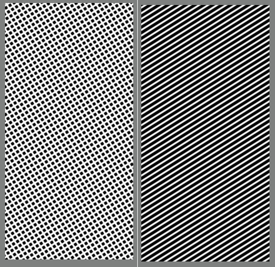
Cellnoise
# Basic usage of the inbuilt seexpr cellnoise function.
# This is based on the prman cellnoise function

# UV vector manipulation
# ----------------------

# Construction of the UV vector. $u and $v are the normalized x and y coordinates for the image. This gives non-square results by default, so we calculate the ratio and then multiply the relevant dimension with said ratio to get a square result from the algorithms.
# The zCoordinate can be set manually in many of the inbuilt noise functions, as these produce 3d noise, but we have a 2d plane. So allowing people to manipulate the last dimension manually allows them to access other slices of the 3d noise.

$ratio = $h/$w;
$zCoord = 0; #0.0, 1.0
$uv = [$u, $v*$ratio, zCoord];

# We multiply the subdivisions with the uv vector to give a sense of zooming out.

$subdivisions = 67; # 1, 100;
$uv *= $subdivisions;

# We also rotate the uv coordinate around the z-axis, [0,0,1].

$rotation = 0; #0, 359;
$uv = rotate($uv, [0,0,1], rad(rotation));


# Cellnoise Function
# ------------------


# Finally we input all the UV into the function to get a factor.
$fac = cellnoise($uv);


# Color
# -----
# We put the factor into a gradient to get the color.

$color = ccurve($fac,0,[0.141,0.059,0.051],4,0.709957,[0.996078,1,0.572549],4,1,[0.976,0.976,0.976],4,0.320346,[0.713725,0.427451,0.647059],4);

# return the color.
$color
Fractal Brownian Motion
# Basic usage of the inbuilt seexpr FBM function.
# This just exposes each of the variables in the FBM function for editing. Also adds rotation and scaling.

# UV vector manipulation
# ----------------------

# Construction of the UV vector. $u and $v are the normalized x and y coordinates for the image. This gives non-square results by default, so we calculate the ratio and then multiply the relevant dimension with said ratio to get a square result from the algorithms.
# The zCoordinate can be set manually in many of the inbuilt noise functions, as these produce 3d noise, but we have a 2d plane. So allowing people to manipulate the last dimension manually allows them to access other slices of the 3d noise.

$ratio = $h/$w;
$zCoord = 0; #0.0, 1.0
$uv = [$u, $v*$ratio, zCoord];

# We multiply the subdivisions with the uv vector to give a sense of zooming out.

$subdivisions = 23; # 1, 100;
$uv *= $subdivisions;

# We also rotate the uv coordinate around the z-axis, [0,0,1].

$rotation = 0; #0, 359;
$uv = rotate($uv, [0,0,1], rad(rotation));


# FBM Function
# ----------------

# Controls the frequencies.
$fbmOctaves = 2; #0, 10

# Spacing between the frequencies - a value of 2 means each octave is twice the previous frequency.
$fbmLacunarity = 1; #0, 10;

# controls how much each frequency is scaled relative to the previous frequency.
$fbmGain = 0.5; #0, 10.0

# Finally we input all the variables into the function to get a factor.
$fac = fbm($uv, $fbmOctaves, $fbmLacunarity, $fbmGain);


# Color
# -----
# We put the factor into a gradient to get the color.

$color = ccurve($fac,0,[0.141,0.059,0.051],4,0.709957,[0.556863,1,0.913725],4,1,[0.976,0.976,0.976],4,0.212121,[0.105882,0.164706,0.266667],4);

# return the color.
$color
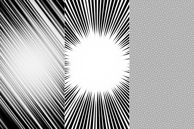
Turbulence
# Basic usage of the inbuilt seexpr turbulence function.
# This just exposes each of the variables in the turbulence function for editing. Also adds rotation and scaling.

# UV vector manipulation
# ----------------------

# Construction of the UV vector. $u and $v are the normalized x and y coordinates for the image. This gives non-square results by default, so we calculate the ratio and then multiply the relevant dimension with said ratio to get a square result from the algorithms.
# The zCoordinate can be set manually in many of the inbuilt noise functions, as these produce 3d noise, but we have a 2d plane. So allowing people to manipulate the last dimension manually allows them to access other slices of the 3d noise.

$ratio = $h/$w;
$zCoord = 0; #0.0, 1.0
$uv = [$u, $v*$ratio, zCoord];

# We multiply the subdivisions with the uv vector to give a sense of zooming out.

$subdivisions = 23; # 1, 100;
$uv *= $subdivisions;

# We also rotate the uv coordinate around the z-axis, [0,0,1].

$rotation = 0; #0, 359;
$uv = rotate($uv, [0,0,1], rad(rotation));


# Tubulence Function
# ------------------

# Controls the frequencies.
$fbmOctaves = 2; #0, 10

# Spacing between the frequencies - a value of 2 means each octave is twice the previous frequency.
$fbmLacunarity = 1; #0, 10;

# controls how much each frequency is scaled relative to the previous frequency.
$fbmGain = 0.5; #0, 10.0

# Finally we input all the variables into the function to get a factor.
$fac = turbulence($uv, $fbmOctaves, $fbmLacunarity, $fbmGain);


# Color
# -----
# We put the factor into a gradient to get the color.

$color = ccurve($fac,0,[0.141,0.059,0.051],4,0.709957,[0.980392,0.662745,1],4,1,[0.976,0.976,0.976],4,0.212121,[0.105882,0.164706,0.266667],4);

# return the color.
$color
And the same song, but now it’s the colornoise functions.
Color Voronoi
# Basic usage of the inbuilt seexpr color voronoi function.
# This just exposes each of the variables in the voronoi function for editing. Also adds rotation and scaling.

# UV vector manipulation
# ----------------------

# Construction of the UV vector. $u and $v are the normalized x and y coordinates for the image. This gives non-square results by default, so we calculate the ratio and then multiply the relevant dimension with said ratio to get a square result from the algorithms.
# The zCoordinate can be set manually in many of the inbuilt noise functions, as these produce 3d noise, but we have a 2d plane. So allowing people to manipulate the last dimension manually allows them to access other slices of the 3d noise.

$ratio = $h/$w;
$zCoord = 0; #0.0, 1.0
$uv = [$u, $v*$ratio, zCoord];

# We multiply the subdivisions with the uv vector to give a sense of zooming out.

$subdivisions = 10; # 1, 100;
$uv *= $subdivisions;

# We also rotate the uv coordinate around the z-axis, [0,0,1].

$rotation = 0; #0, 359;
$uv = rotate($uv, [0,0,1], rad(rotation));


# Voronoi Function
# ----------------

# The type of voronoi algorithm as explain in the manual.
$type = 1; #1, 5

# The jitter, low jitter gives almost grid like appearance, high jitter a
$jitter = 1; #0.0, 1.0

# Some variables for introducing some fractal brownian motion into the voronoi cells.

# The strength of the FBM effect.
$fbmScale = 0.21533;

# Controls the frequencies.
$fbmOctaves = 4; #0, 10

# Spacing between the frequencies - a value of 2 means each octave is twice the previous frequency.
$fbmLacunarity = 2; #0, 10;

# controls how much each frequency is scaled relative to the previous frequency.
$fbmGain = 0.5; #0, 10.0

# Color
# -----
# We put all the variables into the color voronoi function to get the color.

$color = cvoronoi($uv, $type, $jitter, $fbmScale, $fbmOctaves, $fbmLacunarity, $fbmGain);

# return the color.
$color
Color Perlin Noise 1983
# Basic usage of the inbuilt seexpr color noise function.
# This is based on the original 1983 perlin noise.

# UV vector manipulation
# ----------------------

# Construction of the UV vector. $u and $v are the normalized x and y coordinates for the image. This gives non-square results by default, so we calculate the ratio and then multiply the relevant dimension with said ratio to get a square result from the algorithms.
# The zCoordinate can be set manually in many of the inbuilt noise functions, as these produce 3d noise, but we have a 2d plane. So allowing people to manipulate the last dimension manually allows them to access other slices of the 3d noise.

$ratio = $h/$w;
$zCoord = 0; #0.0, 1.0
$uv = [$u, $v*$ratio, zCoord];

# We multiply the subdivisions with the uv vector to give a sense of zooming out.

$subdivisions = 67; # 1, 100;
$uv *= $subdivisions;

# We also rotate the uv coordinate around the z-axis, [0,0,1].

$rotation = 0; #0, 359;
$uv = rotate($uv, [0,0,1], rad(rotation));


# Function
# --------
# Finally we input the UV into the color function to get a color.

$color = cnoise($uv);

# return the color.
$color
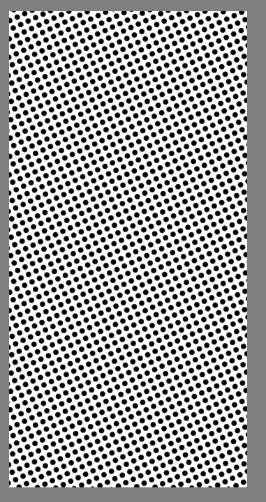
Color Cellnoise
# Basic usage of the inbuilt seexpr color cellnoise function.
# This is based on the prman cellnoise function

# UV vector manipulation
# ----------------------

# Construction of the UV vector. $u and $v are the normalized x and y coordinates for the image. This gives non-square results by default, so we calculate the ratio and then multiply the relevant dimension with said ratio to get a square result from the algorithms.
# The zCoordinate can be set manually in many of the inbuilt noise functions, as these produce 3d noise, but we have a 2d plane. So allowing people to manipulate the last dimension manually allows them to access other slices of the 3d noise.

$ratio = $h/$w;
$zCoord = 0; #0.0, 1.0
$uv = [$u, $v*$ratio, zCoord];

# We multiply the subdivisions with the uv vector to give a sense of zooming out.

$subdivisions = 67; # 1, 100;
$uv *= $subdivisions;

# We also rotate the uv coordinate around the z-axis, [0,0,1].

$rotation = 0; #0, 359;
$uv = rotate($uv, [0,0,1], rad(rotation));


# Cellnoise Function
# ------------------

# We input all the uv into the function to get a color.

$color = ccellnoise($uv);

# return the color.
$color
Color Fractal Brownian Motion
# Basic usage of the inbuilt seexpr color FBM function.
# This just exposes each of the variables in the FBM function for editing. Also adds rotation and scaling.

# UV vector manipulation
# ----------------------

# Construction of the UV vector. $u and $v are the normalized x and y coordinates for the image. This gives non-square results by default, so we calculate the ratio and then multiply the relevant dimension with said ratio to get a square result from the algorithms.
# The zCoordinate can be set manually in many of the inbuilt noise functions, as these produce 3d noise, but we have a 2d plane. So allowing people to manipulate the last dimension manually allows them to access other slices of the 3d noise.

$ratio = $h/$w;
$zCoord = 0; #0.0, 1.0
$uv = [$u, $v*$ratio, zCoord];

# We multiply the subdivisions with the uv vector to give a sense of zooming out.

$subdivisions = 23; # 1, 100;
$uv *= $subdivisions;

# We also rotate the uv coordinate around the z-axis, [0,0,1].

$rotation = 0; #0, 359;
$uv = rotate($uv, [0,0,1], rad(rotation));


# FBM Function
# ----------------

# Controls the frequencies.
$fbmOctaves = 2; #0, 10

# Spacing between the frequencies - a value of 2 means each octave is twice the previous frequency.
$fbmLacunarity = 1; #0, 10;

# controls how much each frequency is scaled relative to the previous frequency.
$fbmGain = 0.5; #0, 10.0


# Color
# -----
# Finally we input all the variables into the function to get a color.

$color = cfbm($uv, $fbmOctaves, $fbmLacunarity, $fbmGain);

# return the color.
$color
Color Turbulence
# Basic usage of the inbuilt seexpr color turbulence function.
# This just exposes each of the variables in the turbulence function for editing. Also adds rotation and scaling.

# UV vector manipulation
# ----------------------

# Construction of the UV vector. $u and $v are the normalized x and y coordinates for the image. This gives non-square results by default, so we calculate the ratio and then multiply the relevant dimension with said ratio to get a square result from the algorithms.
# The zCoordinate can be set manually in many of the inbuilt noise functions, as these produce 3d noise, but we have a 2d plane. So allowing people to manipulate the last dimension manually allows them to access other slices of the 3d noise.

$ratio = $h/$w;
$zCoord = 0; #0.0, 1.0
$uv = [$u, $v*$ratio, zCoord];

# We multiply the subdivisions with the uv vector to give a sense of zooming out.

$subdivisions = 23; # 1, 100;
$uv *= $subdivisions;

# We also rotate the uv coordinate around the z-axis, [0,0,1].

$rotation = 0; #0, 359;
$uv = rotate($uv, [0,0,1], rad(rotation));


# Tubulence Function
# ------------------

# Controls the frequencies.
$fbmOctaves = 2; #0, 10

# Spacing between the frequencies - a value of 2 means each octave is twice the previous frequency.
$fbmLacunarity = 1; #0, 10;

# controls how much each frequency is scaled relative to the previous frequency.
$fbmGain = 0.5; #0, 10.0


# Color
# -----
# We put the factor into the color turbulence to get the color.

$color = cturbulence($uv, $fbmOctaves, $fbmLacunarity, $fbmGain);

# return the color.
$color


 I also really like the setting you expose on the top GUI; “size, repeat, color1 and color 2”. This is exactly the type of preset I would love to get in a list.
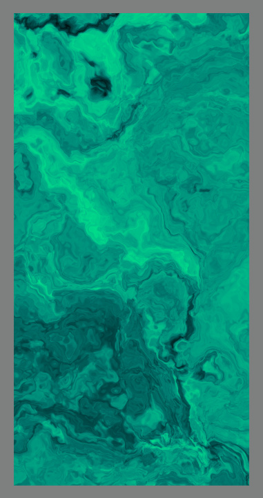


